Recovering a sampled signal • Gabriel I. Alonso

Abstract. A synthetic signal reconstructed from 24 noisy measurements. A Fourier basis models its shape, and a smoothness penalty controls how closely the fit follows noise.

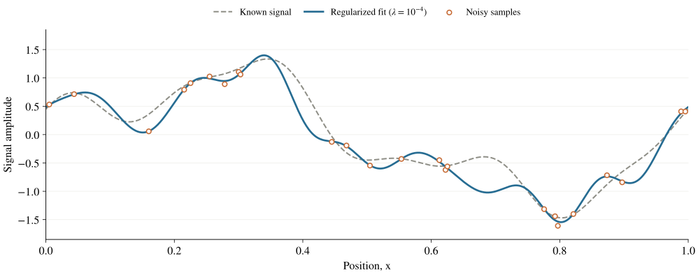
A blue regularized curve follows the gray dashed known signal, passing near 24 orange outlined noisy sample points. — **Figure 1.**
**Reconstruction from noisy samples.** The blue curve retains the broad shape of the known signal while smoothing the noisy measurements. Differences remain in regions with few samples.

1. Introduction

Measurements show only part of a signal. Here, we reconstruct the gaps with a Fourier basis and test how regularization affects the result.

The known signal is sampled at 24 positions in $[0,1]$ . We add Gaussian noise with standard deviation $0.12$ and fit 21 Fourier coefficients. A close fit to the samples can still miss the underlying shape.

2. Method

We write the signal as $f(x)=\sum_{j=0}^{20}c_j\phi_j(x)$ , using a constant term and ten sine–cosine pairs. The sampling matrix $A$ evaluates these 21 basis functions at each measurement position.

\begin{aligned} \mathbf y &= A\mathbf c + \boldsymbol\varepsilon,\\ \boldsymbol\varepsilon &\sim\mathcal N(0,\sigma^2 I). \end{aligned} \tag{1}

We recover the coefficients by balancing the data fit with a penalty on high frequencies:

\begin{aligned} \widehat{\mathbf c}&=\underset{\mathbf c}{\operatorname{argmin}}\;E(\mathbf c),\\ E(\mathbf c)&=\lVert A\mathbf c-\mathbf y\rVert_2^2 +\lambda\mathbf c^{\mathsf T}R\mathbf c. \end{aligned} \tag{2}

The diagonal entries of $R$ are $k^4$ for frequency $k$ ; the constant term is unpenalized. Higher frequencies therefore cost more. For $\lambda>0$ , the solution satisfies

\left(A^{\mathsf T}A+\lambda R\right)\widehat{\mathbf c} =A^{\mathsf T}\mathbf y. \tag{3}

The parameter $\lambda$ controls the tradeoff: a small value leaves oscillations, while a large value removes detail. Equation (2) and Figure 1 show that choice in two forms.

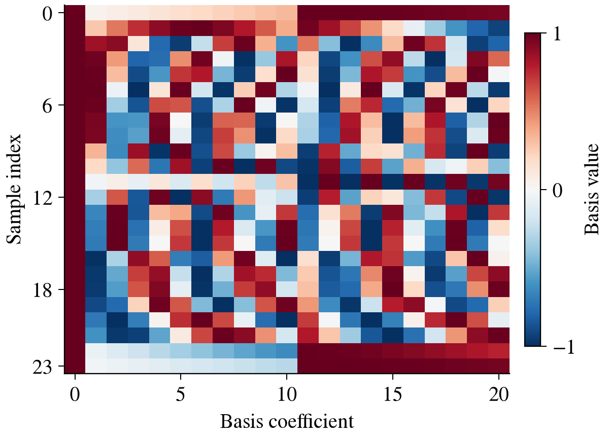
A red and blue heat map of the 24 by 21 sampling matrix. Each row is a sample position and each column is a Fourier basis coefficient. — **Figure 2.** The sampling matrix. Each row evaluates the 21 basis functions at one measurement position.

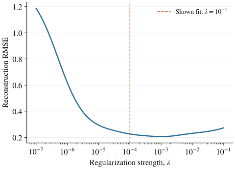
Reconstruction error decreases as regularization increases, reaches a minimum, then rises. An orange dashed line marks the illustrated regularization strength of ten to the minus four. — **Figure 3.** Error across regularization strengths. The dashed line marks the fit shown in Figure 1; it is an illustrative choice, rather than the minimum of this curve.

3. Results

The regularized reconstruction in Figure 1 has a root mean square error of $0.2265$ , compared with $1.3724$ for the unregularized fit. These errors are evaluated against the known signal on a dense grid, rather than at the noisy sample positions.¹

The lowest error occurs at $\lambda=10^{-3}$ (Table 1), a stronger setting than Figure 1 uses. The smoother fit reduces average error while changing some smaller features.

Table 1. Reconstruction error for the same 24 measurements. Lower values indicate a closer fit to the known signal.

Regularization, λ	RMSE
0 (unregularized)	1.3724
0.00001	0.2939
0.00010	0.2265
0.00100	0.2067

4. Writing a paper

Write in Markdown with LaTeX math: $...$ inline and $$...$$ for equations. Figures and tables use one column by default; add wide for both. Wide blocks sit above the text, or below it with placement="bottom". Add <PageBreak /> for another sheet.

Copy the paper template, then set your title, authors, abstract, and date. Use pdf to link an existing paper. Formatting is prepared during the build, so the page works with JavaScript disabled.

5. Code

The reconstruction is a small linear solve. Use least squares for the unregularized case and solve the penalized system when $\lambda>0$ .

import numpy as np

def reconstruct(
    A, B, y, k, strength
):
    weights = np.r_[0, k**4, k**4]
    penalty = np.diag(weights)
    if strength == 0:
        c = np.linalg.lstsq(
            A, y, rcond=None
        )[0]
    else:
        system = (
            A.T @ A + strength * penalty
        )
        c = np.linalg.solve(
            system, A.T @ y
        )
    return B @ c

The figure generation script contains the signal, samples, plots, and table values. It uses a fixed random seed so the example can be reproduced.

Footnotes

The known signal is available because this is a synthetic example. In an actual inverse problem, evaluation requires independent evidence or held out measurements. ↩